Phonetic vowel charts in LaTeX
🕑 12 min • 👤 Thomas Graf • 📆 August 26, 2020 in Tutorials • 🏷 student advice, LaTeX, phonetics
It’s nice to have loyal readers. One of them wrote me an email a few days ago that starts as follows:
Hi, hope all is well with you. I notice Outdex has been silent for longer than usual but I prefer to assume that that is because you are doing something more fun.
Guilty as charged. In anticipation of my 1-year sabbatical (*gloat*), I have used this summer for an extended vacation from everything linguistics and academia. Well, not quite, there was something fun I did that is sort of related to linguistics, but more on that in an upcoming post. Anyway, this loyal reader knows how to reel me back in: a LaTeX question! More precisely, the best way to typeset a vowel chart in tikz, which is the standard solution for graphics in LaTeX nowadays. Challenge accepted.
The task
Typesetting a vowel chart in tikz isn’t particularly hard, but this specific request comes with a few additional design desiderata. First, the placement of the vowels should be fairly accurate, ideally by using F1 and F2 frequencies as is commonly done in the literature.
Second, it should be possible to easily highlight variations between dialects, e.g. by showing dialect A in red, dialect B in blue, and connecting their peripheral vowels in a path. Third, it should be possible to transform the F1/F2-based chart so that it looks more like the idealized trapezoid in the IPA chart.
General observations
It’s tempting to just rush in and write some tikz code right away, but hold your horses. First let’s decide if tikz is the right tool for this. Does tikz make it easy to accurately place nodes? Yes, but it’s tedious if there’s many nodes. Now, does tikz make it easy to connect nodes with lines? Again, it’s not hard, but it’s manual work. Finally, does tikz allow us to apply transformations to an image so that it becomes more trapezoid? Yes, but it’s decidedly not easy. So tikz doesn’t look like the right tool for this.
Fortunately, tikz has a companion package that checks all boxes, and that’s pgfplots. Both tikz and pgfplots use the pgf library to produce graphics, and they are interoperable. But whereas tikz is a general purpose solution for graphics in LaTeX, pgfplots is designed just for creating plots. It makes it very easy to plot data in LaTeX: you feed in a file of data points, e.g. formant frequencies, and out comes a nice plot. It can be a scatter plot that only shows dots, or your typical line and bar plots. Thanks to those features, pgfplots should be able to take care of points 1 and 2 without much effort.
This leaves us with requirement 3, the transformations. This isn’t handled directly by pgfplots. But since the data can be stored externally in a separate file, you can change the plot by changing the data points in that file. And for that you can use any tool you want, be it Python, R, Julia, Matlab, bash, whatever. And of course you can also do it manually. That’s arguably the most flexible solution, but if you still want to use tikz transformations you can do that because tikz and pgfplots interact seemlessly (remember, they’re both high-level tools for working with pgf).
Okay, pgfplots it is, then. Let’s see how it’s done.
Building a plot step by step
Setting up
We start out with a new .tex file and drop in some boilerplate code.
\documentclass[tikz,crop]{standalone}

\usepackage{pgfplots}
\pgfplotsset{compat=newest}

\usepackage[utf8]{inputenc}
\usepackage[charter]{mathdesign}

\begin{document}
\end{document}
This doesn’t do anything yet. I use the standalone class with the options [tikz,crop] so that LaTeX loads tikz and produces a pdf that is the size of the produced image. If I had used the article class, I would have gotten a single page in letter size with the image at the top — not as nice to work with. There’s several other advantages to doing this as a standalone document, but I suppose that’s best left for a future post.
After this, I load pgfplots and use \pgfplotsset{compat=newest} to tell it to use the most up-to-date version of its syntax. Then I tell LaTeX that the file uses the standard unicode text encoding, and I load the Charter font because I like it.
Adding a simple plot
Now we add a simple plot, loading data from a file mydata.dat. The document section has to be expanded as follows:
\begin{document}
\begin{tikzpicture}
    \begin{axis}
        \addplot table {mydata.dat};
    \end{axis}
\end{tikzpicture}
\end{document}
Notice the multiple levels of nesting here: We create a tikz picture, which will consists of a pgfplot (the axis environment), and in this plot we can map data points via the \addplot command. In the case at hand, we load a single set of data points from a table in the file mydata.dat, which must be in the same directory as our tex-file.
To keep this example self-contained, however, I’ll instead add the data directly to the tex-file. This can be done with the filecontents package.
\documentclass[tikz,crop]{standalone}

\usepackage{pgfplots}
\pgfplotsset{compat=newest}
\usepackage{filecontents}

\usepackage[utf8]{inputenc}
\usepackage[charter]{mathdesign}

\begin{filecontents}{mydata.dat}
x        y
2400     240
2300     390
2100     235
1900     370
1900     610
1710     585
1610     850
1530     820
940      750
760      700
1170     600
700      500
1310     460
640      360
595      250
\end{filecontents}


\begin{document}
\begin{tikzpicture}
    \begin{axis}
        \addplot table {mydata.dat};
    \end{axis}
\end{tikzpicture}
\end{document}
Now the code contains a filecontents environment before \begin{documents}. Inside the environment is a whitespace-separated table of formant frequencies for various vowels. I have labeled the columns x and y for easier use with pgfplots. During compilation, LaTeX will write this table to the file mydata.dat, which is then read by pgfplots to construct the plot. The final result is shown below.

Okay, that was easy. If all you want is a simple line plot, you’re done. But we want more, so let’s keep pushing.
Switching from lines to dots
While we do want the ability to connect the dots in the plot with lines, we also want to construct a normal vowel chart. So all the different dots shouldn’t be connected by a line (yet). Time to tweak the plot:
\begin{tikzpicture}
    \begin{axis}
        \addplot[
        only marks,
        ] table {mydata.dat};
    \end{axis}
\end{tikzpicture}
Can you spot the difference? We have expanded \addplot to \addplot[only marks,], which instructs pgfplots not to connect the data points with a line.

Labeling the axes
The plot isn’t particularly informative yet because a person looking at it has no idea what the axes encode, nor what each point denotes. We’ll handle this in two steps. Let’s start with the axis labels because those are way easier.
\begin{document}
\begin{tikzpicture}
    \begin{axis}[
        xlabel={F2},
        ylabel={F1},
        ]
        \addplot[
        only marks,
        ] table {mydata.dat};
    \end{axis}
\end{tikzpicture}
\end{document}
Two more options have been added, xlabel and ylabel. But this time they go with the axis-environment rather than \addplot. That’s because these parameters affect the whole plot, not just a specific set of data points. With these modifications, you’ll now get the following plot.

Hardly a big change, what we really need is labels for the individual data points.
Labeling the data points
This is perhaps the most complicated part of the code, and it involves several interacting parts. First, we have to change the table so that it also specifies the label for each data point.
\begin{filecontents}{mydata.dat}
x        y       label
2400     240     i
2300     390     e
2100     235     y
1900     370     {\o}
1900     610     E
1710     585     {\oe}
1610     850     a
1530     820     {\ae}
940      750     A
760      700     6
1170     600     v
700      500     O
1310     460     Y
640      360     o
595      250     u
\end{filecontents}
I have chosen label names that will work well with tipa, the LaTeX package for IPA notation.
Next we have to tell pgfplots what it should do with this label. That’s the tricky part. How about you look at the full code first and try to figure out what’s going on.
\begin{document}
\begin{tikzpicture}
    \begin{axis}[
        xlabel={F2},
        ylabel={F1},
        %
        visualization depends on={value \thisrow{label} \as \thelabel},
        every node near coord/.append style={%
            label={\textipa{\thelabel}},
            }
        ]
        \addplot[
        only marks,
        nodes near coords,
        ] table {mydata.dat};
    \end{axis}
\end{tikzpicture}
\end{document}
This code makes more sense when read in reverse. The \addplot command has been expanded with a second option nodes near coords. This is the standard pgfplots way for adding a label to each data point. But pgfplots’ default style for this isn’t quite what we want, so we also add a new piece of code to the axis environment:
This says that nodes that are added because of the nodes near coords option should have their style modified so that the label is the output of \textipa{\thelabel} — basically, the IPA label! But this still isn’t quite enough because \thelabel isn’t a default command, it needs to be defined. That’s what the line immediately above does.
In plain English: for each data point, \thelabel refers to its value in the label column. So overall, we had to add three lines of code to get labels. But surely the reward of a fully labeled vowel chart will be worth it, right?

Looks like we forgot something…
Fixing the data point labels
We want the data point labels to be just the IPA symbols, but pgfplots somehow decided to print both the F1-frequency and the IPA symbol. And we would also like the data points to still be, well, points.
In order to fix this, we have to add the option point meta=explicit symbolic to the axis-environment. This basically tells pgfplots to only use the explicitly provided label and nothing else. And we also have to add scatter to \addplot so that pgfplot knows that we’re arranging these data points as a scatter plot, and in scatter plots each data point still has to be shown as an actual dot even if we’re displaying labels.
\begin{document}
\begin{tikzpicture}
\begin{axis}[
xlabel={F2},
ylabel={F1},
%
point meta=explicit symbolic,
visualization depends on={value \thisrow{label} \as \thelabel},
every node near coord/.append style={%
    label={\textipa{\thelabel}},
    }
]
\addplot[
only marks,
nodes near coords,
] table {mydata.dat};
\end{axis}
\end{tikzpicture}
\end{document}
Changing the origin
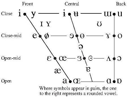
Now that we have nicely labeled dots, we can see that the vowels aren’t arranged in the way we would have expected. For instance, i is in the bottom right instead of the top left, and u is in the bottom left instead of the top right. If you contrast our plot against the one from Wikipedia at the top of this post, you can easily spot the problem. Our plot puts the origin (0,0) in the bottom left, whereas the Wikipedia plot has it in the top right. Or, putting it in clunkier terms, the Wikipedia plot reverses the direction of the axes.
These clunkier terms are exactly the ones used by pgfplots — x dir=reverse and y dir=reverse. Again these options go on the axis-environment because they affect the whole plot.
\begin{document}
\begin{tikzpicture}
    \begin{axis}[
        xlabel={F2},
        ylabel={F1},
        x dir=reverse,
        y dir=reverse,
        %
        point meta=explicit symbolic,
        visualization depends on={value \thisrow{label} \as \thelabel},
        every node near coord/.append style={%
            label={\textipa{\thelabel}},
            }
        ]
        \addplot[
        scatter,
        only marks,
        nodes near coords,
        ] table {mydata.dat};
    \end{axis}
\end{tikzpicture}
\end{document}
This still doesn’t look right, though. The numbers now grow in reverse, as desired, but they’re still drawn on the left edge for the y-axis and the bottom edge for the x-axis. That’s very confusing. We have to tell pgfplots that it shouldn’t just reverse the direction of the axes, it should also place each one at the opposite edge. That’s what axis x line* and axis y line* are for.
\begin{document}
\begin{tikzpicture}
    \begin{axis}[
        xlabel={F2},
        ylabel={F1},
        x dir=reverse,
        y dir=reverse,
        axis x line*=top,
        axis y line*=right,
        %
        point meta=explicit symbolic,
        visualization depends on={value \thisrow{label} \as \thelabel},
        every node near coord/.append style={%
            label={\textipa{\thelabel}},
            }
        ]
        \addplot[
        scatter,
        only marks,
        nodes near coords,
        ] table {mydata.dat};
    \end{axis}
\end{tikzpicture}
\end{document}
Controlling label placement
We basically have a fully readable plot now, but it doesn’t look all that nice. For instance, the vowels i and y are placed on top of the F2-axis. And where vowels are placed closely together, it is easy to confuse the labels. We need more fine-grained control over the labels. While there’s many ways this could be done, I’ll present one that’s fairly flexible and primarily relies on techniques already covered in this tutorial.
First, we once again modify the style of nodes near coordinates so that they can are placed at a specific angle from the center of the data point’s dot. So instead of this:
we’ll have this
Notice the addition of \labelangle:, which will take a number and put the label at this specific angle. For instance, if \labelangle is 90, the label will be above the dot, whereas an angle of 270 would put it below the dot. But where does \labelangle get its value from? Well, we have to do it exactly the same way as we did with \thelabel: we put it in the table and use visualization depends on to tell pgfplots how to use the additional data in the table.
\begin{filecontents}{mydata.dat}
x y label angle
2400 240 i 120
2300 390 e 90
2100 235 y 270
1900 370 {\o} 90
1900 610 E 90
1710 585 {\oe} 270
1610 850 a 270
1530 820 {\ae} 0
940 750 A 90
760 700 6 90
1170 600 v 90
700 500 O 90
1310 460 Y 90
640 360 o 90
595 250 u 90
\end{filecontents}
\begin{document}
\begin{tikzpicture}
\begin{axis}[
xlabel={F2},
ylabel={F1},
x dir=reverse,
y dir=reverse,
axis x line*=top,
axis y line*=right,
%
point meta=explicit symbolic,
visualization depends on={value \thisrow{label} \as \thelabel},
visualization depends on={value \thisrow{angle} \as \labelangle},
every node near coord/.append style={%
    anchor=center,
    label={\labelangle:\textipa{\thelabel}},
    }
]
\addplot[
scatter,
only marks,
nodes near coords,
] table {mydata.dat};
\end{axis}
\end{tikzpicture}
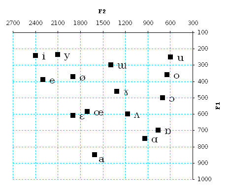
\end{document}The angle values in the table can be tweaked to get the most pleasing placement. Since the placement of the label follows tikz-conventions, we could put all kinds of additional formatting information in the table to style the labels exactly the way we want.

Quite generally, you can use what you know about tikz to modify the output of pgfplots. For instance, we can make the axis labels boldface and rotate them to be more readable.

Final code
The final plot above is produced by the code snippet below:
\documentclass[tikz,crop]{standalone}

\usepackage{pgfplots}
\pgfplotsset{compat=newest}
\usepackage{filecontents}

\usepackage[utf8]{inputenc}
\usepackage[charter]{mathdesign}
\usepackage{tipa}

\begin{filecontents}{mydata.dat}
x        y       label   angle
2400     240     i       120
2300     390     e       90
2100     235     y       270
1900     370     {\o}    90
1900     610     E       90
1710     585     {\oe}   270
1610     850     a       270
1530     820     {\ae}   0
940      750     A       90
760      700     6       90
1170     600     v       90
700      500     O       90
1310     460     Y       90
640      360     o       90
595      250     u       90
\end{filecontents}


\begin{document}
\begin{tikzpicture}
    \begin{axis}[
        xlabel={F2},
        ylabel={F1},
        x label style={font=\bfseries,anchor=south},
        y label style={font=\bfseries,rotate=-90,anchor=west},
        x dir=reverse,
        y dir=reverse,
        axis x line*=top,
        axis y line*=right,
        %
        point meta=explicit symbolic,
        visualization depends on={value \thisrow{label} \as \thelabel},
        visualization depends on={value \thisrow{angle} \as \labelangle},
        every node near coord/.append style={%
            anchor=center,
            label={\labelangle:\textipa{\thelabel}},
            }
        ]
        \addplot[
        scatter,
        only marks,
        nodes near coords,
        ] table {mydata.dat};
    \end{axis}
\end{tikzpicture}
\end{document}
Although it takes a while to get the hang of pgfplots, once you know your way around it’s remarkably easy to produce nice plots. Just as with tikz, the learning curve might not be worth it for everyone, but depending on what you currently use to plot data or draw vowel charts, this might save you quite a bit of time.
Addendum: contrasting dialects
I was just about ready to wrap up this post when I remembered that I should also show off the line graph contrasting two dialects. But guess what: it’s trivially easy. For each dialect, we create a separate table. Here I’m adding two tables dialectA.dat and dialectB.dat. Each one contains the peripheral vowels of that dialect. To keep things easy for me, Dialect B increases both the F1 and the F2 of each sound of Dialect A by 100. If you want to have the tables directly in the LaTeX file, you need two separate filecontents environments.
\begin{filecontents}{dialectA.dat}
x        y       label   angle
2400     240     i       120
2300     390     e       90
1900     610     E       90
1610     850     a       270
940      750     A       90
760      700     6       90
700      500     O       90
640      360     o       90
595      250     u       90
\end{filecontents}

\begin{filecontents}{dialectB.dat}
x        y       label   angle
2500     340     i       120
2400     490     e       90
2000     710     E       90
1700     950     a       270
1040     850     A       90
860      800     6       90
800      600     O       90
740      460     o       90
695      350     u       90
\end{filecontents}
Then you can use almost exactly the same code as the one above, you just have to switch back from scatter plot to the default line plot. Oh, and don’t forget to specify colors for the lines.
\begin{document}
\begin{tikzpicture}
    \begin{axis}[
        xlabel={F2},
        ylabel={F1},
        x label style={font=\bfseries,anchor=south},
        y label style={font=\bfseries,rotate=-90,anchor=west},
        x dir=reverse,
        y dir=reverse,
        axis x line*=top,
        axis y line*=right,
        %
        point meta=explicit symbolic,
        visualization depends on={value \thisrow{label} \as \thelabel},
        visualization depends on={value \thisrow{angle} \as \labelangle},
        every node near coord/.append style={%
            anchor=center,
            label={\labelangle:\textipa{\thelabel}},
            }
        ]
        \addplot[
        red,
        ] table {dialectA.dat};
        \addplot[
        blue,
        ] table {dialectB.dat};
    \end{axis}
\end{tikzpicture}
\end{document}
There you go, easy peasy. Add some custom command magic and tikz styling on top of it, and you can easily produce different types of plots from a single piece of code. That’s the strength of coding based solutions rather than drawing plots by hand or in some GUI: if you put in the work, you can automate it and save yourself time and effort down the road. Assuming, of course, that you do this often enough to be worth the setup, maintenance, and debugging cost.
Comments powered by Talkyard. Having trouble? Check the FAQ!